

The Making of a Software Wind-Tunnel (part 2)
Dynamical similarity and how to scale models
In part 1, I put forward the idea that we might design and test software at scale by understanding how to build scale models, as one does in fluid- and aerodynamics. Putting a model plane in a wind-tunnel is considerably cheaper than testing on a full-size replica as long as we understand the limitations. Similarly, testing software on small infrastructure could be cheaper than testing on a full scale deployment, if we can understand its limits. The aim of this series is to understand those limits and where they come from.
The task I've set here involves surprisingly complex issues, all of which are the normal domain of physicists and engineers in existing disciplines outside of Information Technology, at various levels of difficulty (the ability to scale measurements is used to calculate drug doses in different patients, for example). Without getting very technical, I would like to sketch out the landscape of the methodology. It picks up from the dimensional analysis described in part 1.
Let them eat Buckingham Pi
We all have an intuitive notion of self-similarity when making something. Suppose we make a meal for two, doubling everything could make a meal for four. But, what about the cooking time? Should we double that too? Luckily there is a methodology for working it out.
They key insight in physics of scales is that it is dimensionless ratios of scales that determine important behaviours in the world, not lengths and times directly. This seems reasonable, as only dimensionless ratios are (manifestly) independent of the units used to measure things. It cannot be the case that a phenomenon depends on whether it is measured in centimetres or inches.
The Buckingham Pi Theorem formalizes the notion that only dimensionless scales are useful for characterizing and extrapolating behaviour (for instance, to make a scale model). Any variable that cannot be directly compared to another in the same system of measurements is potentially a fiction of the measurement itself.
The Buckingham method allows us to write behavioural relationships (like flow equations) in a form which depends on on dimensionless combinations of variables. Although this is just a rewriting exercise, it casts relationships in a form that is manifestly free of assumptions about scale. We can only say how big something is relative to a calibration reference; anything else is subjective and subject to ad hoc interpretation.
From any set of parameters, one begins by putting together all the possible dimensionless combinations. For example, in the case of an aspect ratio, a rectangle has width W and height H, both of which have the dimensions of length. So W/H is the only combination. If we add the third dimension, there is distance from the observer to the screen D, so now we can also make W/D, H/D, W/H.

If all of these ratios are the same for the observer, then the observer will not be able to tell the difference between the self-similar rectangles above. This also applies if the something actionable happens, such as, say, you get run over by a train --- the damage done by a smaller train at greater speed would be the same in a dynamically similar system.
This need not be easy. Isolated systems have nice scaling properties but, once connected to the real world, the interaction with other variables complicates matters. Particularly tricky are time-dependent scalings, where some changing flow interacts with more static variables, e.g. the airflow over a wing (hence the value of a wind-tunnel). Dynamical scales can change the balance points of equilibria (e.g. "lift versus gravity") with functional consequences.
Data processing example
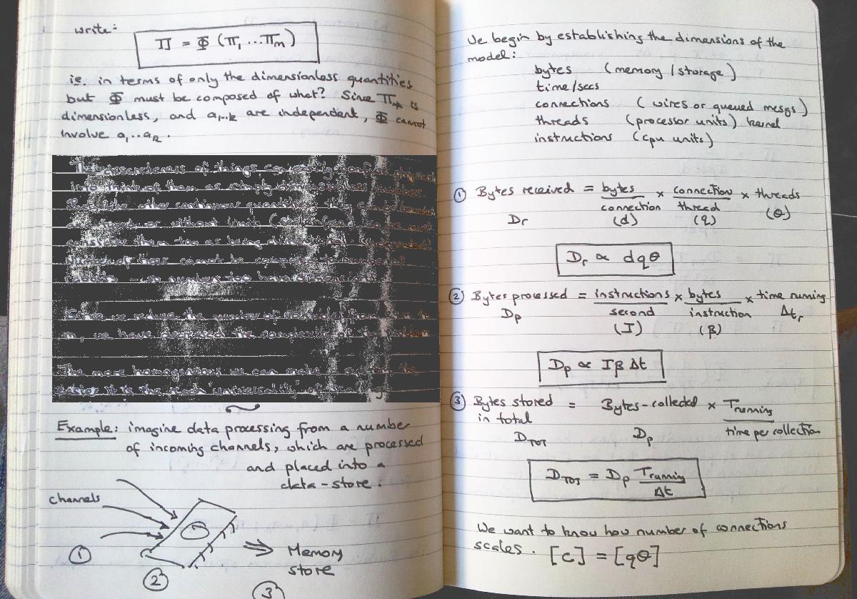
Consider a simple flow example of data processing by collecting data from a number of hosts. We might end up with a very simple model that can be summarized something like this:

| Symbol | Interpretation | Units |
|---|---|---|
| Dtotal | amount of data processed | bytes |
| Trunning | Total running time of process | seconds |
| dc | Data transferred in one connection | bytes per connection |
| ΔT | Time for one round of data | seconds |
| q | Connections per thread | Connections per thread |
| θ | Parallel threads | threads |
Suppose we want to know how the number of connections "c" scales (perhaps because we want to know how many hosts we can support processing data from). The Buckingham Pi theorem says that we look for dimensionless combinations of variables such that a dimensionless version of "c" is a function of the other dimensionless scales in the problem. The dimensionless combinations can be verified:

And we can write the one involving the parameter of interest as a function of the others.

The importance of this is that these ratios must be preserved in order to build a model with the same dynamical behaviour. So if we change say q then to preserve the ratio, we must change say Dtotal or one of the other values to compensate. This means we can choose to reduce expensive or difficult scales by compensating with cheaper changes. If we do this, then the scaling of the number of connections must go like the prefix to the function Φ since Φ is a scale invariant.

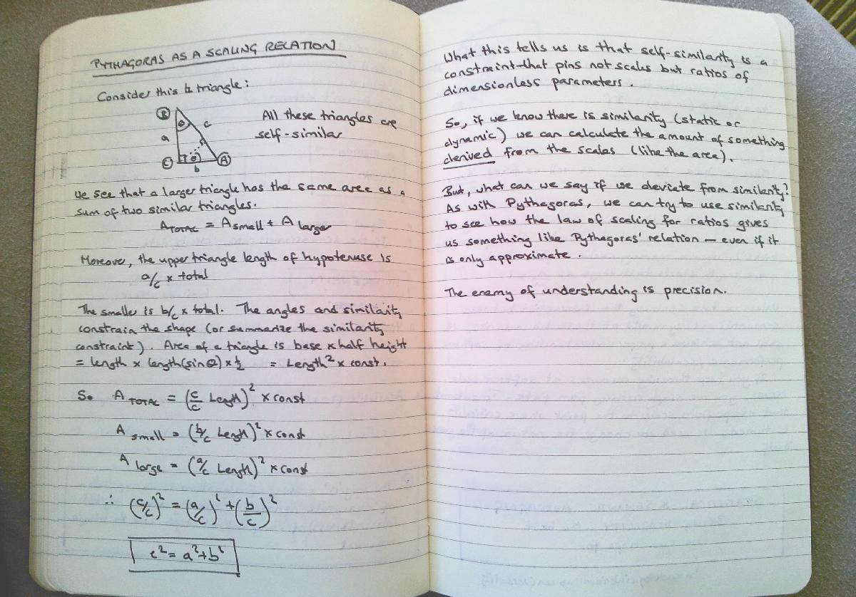
Notice that the dependence on the running time indicates that the connections could, in principle, depend on the time taken for an update. This does not seem likely, and we might be able to eliminate this on other grounds. Dimensional analysis leaves open every possibility for change; it cannot completely pin down a model without additional information in general. Suffice it to say that this kind of analysis is what allows scale models to be used and medicinal dosages to be calculated for patients of different sizes. However, sometimes we can pin down a model---note how we can completely lock down Pythagoras theorem from the self-similarity of right angled triangles).
A longer version of this example, page 1 and page 2 are here in note form for interested readers.
Digilogy: from the discrete to the ridiculous
What this tells us is that self-similarity, or scaling is a form of relativity. Each measurement makes sense relative to another, in the same proportion. As long as we can change the parameters freely, a system can be scaled up or down as much as we like and we can test a smaller model for a larger thing, or vice versa.
There's a catch. This nice picture begins to unravel if there are fixed scales that pin us to a specific size, as mentioned in part 1. There are two ways this can happen:
- The underlying system is composed of discrete building blocks of fixed size, constraining it `from below'.
- There are boundaries that enclose the whole system, constraining it `from above'.
Discreteness (digital/symbolic indivisibility) spoils scaling by fixing a scale. (see figure below). We can scale a model to a larger size, but if both small and large are built from bricks of the same size, then we've pinned a scale. This is true in atomic theory, and it leads to to the so-called continuum approximation in which underlying discreteness vanishes from the picture, and ideas about `renormalization'.

Imagine a car park (parking lot). The size of a car (hence parking space) does not change, it is pinned, so we cannot simply model a parking lot to twice the size, with the same size cars, by scaling all the lengths and times. It would not be a similarity transformation, but a different model altogether.
The caveat is that sometimes we can disregard such scales if their effect on the behaviour of the system can be shown irrelevant. For instance, in a wind-tunnel, we don't need to scale the size of the air atoms by the same ratio as we scale a plane, because the size of atoms is already so much smaller than both plane and model that the difference is completely negligible.
Machine learning of scalability?
Often we just want to know how to scale up and achieve more. The key to success seems to lie in how to approximate. How do we find out what really dominates the behaviour?
Dimensional methods succeed mostly when systems are dominated by simple behaviour. The kind of complexity in modern software far outstrips that of most physical systems. However, we also have the help of computers in managing such information, so there is a way to apply brute force to help manage this. Indeed, if scale awareness could be built into software and languages directly, this could simply be a part of software engineering.
How could software instrumentation help? If we can map out the scaling of all the tiny parts, then there is no reason why a nano-technology approach of handling every detail could not work by brute force in simpler configurations, but the level of sensitivity could then be tuned to design limits. Instrumentation could at least determine if any changes would violate scale invariance, there will only be scale-free behaviour (dynamical similarity) up to the scale of the first violated limit. This will pin the behaviour. We need to know mainly which scales excite resonances and dominate behaviour.
Discrete resources like CPUs, hosts threads, packets, switches, etc can pin. Virtualization can perform sharing across these discrete elements that alters their scaling properties. Finally, there is the issue of how we measure intent. This is where the promise theory enters the picture.
Prospects
The technicalities involved in scaling are intense and we see how fragile the relationships are. There can be so many variables that building a scale model could seem like hubris. But this actually shows us how fragile software itself is to small changes in its environment. If we have any hope of predicting scalability we have to build fundamentally simple things that can be scaled with elementary patterns. The more non-similar moving parts, the less we will be able to promise with certainty.
In Part 3, I want to discuss critical behaviour and scaling catastrophes.